Create Tables from the Fisheries Economics of the US (FEUS) Report

Emily Markowitz (Emily.Markowitz AT NOAA.gov / EmilyMarkowitz-NOAA)

August 24 2021

Create Tables from the Fisheries Economics of the US (FEUS) Report

Purpose: Construct the FEUS Commerical Fisheries state and national tables and output them to csv files

PKG <- c(# devtools::install_github("emilymarkowitz-NOAA/FishEconProdOutput", force = TRUE)
         "FishEconProdOutput",
         
         #Seperating species by taxonomic group
         "taxize",  # install.packages("remotes"); remotes::install_github("ropensci/taxize")
         
         # Data Managment
         "tidyverse",
         "filesstrings", 
         "data.table", 
         "plyr",  
         "dplyr",
         "rlist",
         
         # #RMarkdown
         "rmarkdown",
         "ggpubr",
         "kableExtra",
         
         #Excel File Management
         "xlsx",
         "readxl"
)

for (p in PKG) {
  if(!require(p,character.only = TRUE)) {  
    install.packages(p, repos = "http://cran.us.r-project.org")
    require(p,character.only = TRUE)}
}

1. Set knowns

# Define what regions we are interested in
reg_order = c("National", "North Pacific", "Pacific", "Western Pacific (Hawai`i)", 
              "New England", 
              "Mid-Atlantic", "South Atlantic", "Gulf of Mexico")

reg_order_abbrv = c("US", "NP", "Pac", "WP", "NE", "MA", "SA", "GOM")

# Define Category
category0 = "category"

# Define Years
maxyr<-2018
yr <- minyr <- minyr.data<-as.numeric(paste0(floor((maxyr-24)/10), 
                              ifelse(substr(maxyr, start = nchar((maxyr-24)), 
                                            stop = nchar((maxyr-24)))>=5, 6, 1))) #of data going into the analysis
minyr.ProdOut<-maxyr-19 # That will be shown in the analysis
baseyr<-as.numeric(paste0(floor(maxyr/10), 
                          ifelse(substr(maxyr, start = nchar(maxyr), 
                                        stop = nchar(maxyr))>=5, 5, 0))) #Will change every 5 years, e.g., maxyr 2019 = byr 2015; maxyr 2020 = byr 2020; maxyr 2021 = byr 2020

2. Set your directories where you will save everything

  
# Folder name for output
folder<-"T567_ProdOutput"
titleadd = paste0(minyr.ProdOut, "To", maxyr, "_FSFEUS")
counter<-0
  
dir_in<-getwd()

if (TF) {
  #Local Directories
  dir_outputtables<-paste0(dir_in, "/output/")
  dir.create(dir_outputtables)

  # Define Directories
  dir_analyses = paste0(dir_outputtables, folder)
  dir.create(dir_analyses)
} else {
  dir_analyses<-dir_outputtables<-dir_in
}

3. Load example data

counter<-0
landings_data<-FishEconProdOutput::land
landings_data$category<-NULL # for this example, let's pretend that this column doesn't already exist
knitr::kable(head(landings_data), booktabs = T) %>%
  kable_styling(latex_options = "striped")

	Year	Pounds	Dollars	Tsn	State	Region	abbvreg
5	2001	613	750	83677	Oregon	Pacific	Pac
6	2003	172	119	83677	Oregon	Pacific	Pac
7	2006	131	131	83677	North Carolina	South Atlantic	SA
14	2005	15	30	83677	Maryland	Mid-Atlantic	MA
15	2004	3	2	83677	New Jersey	Mid-Atlantic	MA
16	2006	37	28	83677	New Jersey	Mid-Atlantic	MA

4. Use itis_reclassify() to categorize all of the species

This can take a minute!

temp <- itis_reclassify(tsn = unique(landings_data$Tsn), 
                 categories = list('Finfish' = c(914179, #  Infraphylum Gnathostomata
                                                -914181), # Tetrapoda; - = do NOT include
                                   "Shellfish" = c(82696, # Phylum  Arthropoda
                                                   69458)), # Phylum    Mollusca
                 uncategorized_name = "uncategorized")

tsn_id<-temp$df_out

# Remove anything that wasn't classified (we don't them for what we are doing here)
if (sum(tsn_id$category %in% c("Other", "Uncategorized"))>0) {
  tsn_id<-tsn_id[!(tsn_id$category %in% c("Other", "Uncategorized")), 
                 c("TSN", "category")]
}

# renaming columns for joining other datasets to this dataset
landings_data<-dplyr::rename(landings_data, 
                 TSN = Tsn)

tsn_id$TSN<-as.numeric(tsn_id$TSN)

# Join the FOSS landings data to their respctive categories
landings_data<-dplyr::left_join(x = landings_data, 
                    y = tsn_id, 
                    by = "TSN")

# Rename columns so they match what the funciton uses
landings_data<-dplyr::rename(landings_data, 
                 Tsn = TSN)

knitr::kable(head(landings_data), booktabs = T) %>%
  kable_styling(latex_options = "striped")

Year	Pounds	Dollars	Tsn	State	Region	abbvreg	category	valid	rank	sciname
2001	613	750	83677	Oregon	Pacific	Pac	Shellfish	valid	subphylum	Crustacea
2003	172	119	83677	Oregon	Pacific	Pac	Shellfish	valid	subphylum	Crustacea
2006	131	131	83677	North Carolina	South Atlantic	SA	Shellfish	valid	subphylum	Crustacea
2005	15	30	83677	Maryland	Mid-Atlantic	MA	Shellfish	valid	subphylum	Crustacea
2004	3	2	83677	New Jersey	Mid-Atlantic	MA	Shellfish	valid	subphylum	Crustacea
2006	37	28	83677	New Jersey	Mid-Atlantic	MA	Shellfish	valid	subphylum	Crustacea

5. Run Analysis

out <- OutputAnalysis(landings_data = landings_data, 
               category0 = category0, # the name of the column you are categorizing by
               baseyr = baseyr, 
               titleadd = titleadd, 
               dir_analyses = dir_analyses, 
               skipplots = TRUE, 
               reg_order = reg_order, # The region(s) you want to assess
               reg_order_abbrv = reg_order_abbrv, # The region(s) you want to assess
               save_outputs_to_file = TF) # Here I use the variable TF so I can change it once at the begining of my code, depending on my reporting purposes
#> [1] "National"
#> [1] "North Pacific"
#> [1] "Pacific"
#> [1] "Western Pacific (Hawai`i)"
#> [1] "New England"
#> [1] "Mid-Atlantic"
#> [1] "South Atlantic"
#> [1] "Gulf of Mexico"
#> [1] "Create spreadsheets"
#> [1] "Create plots"

names(out)
#> [1] "warnings_list"    "editeddata_list"  "index_list"       "spp_list"        
#> [5] "figures_list"     "gridfigures_list"

for (jjj in 1:length(out)) {
  assign(names(out)[jjj], out[[jjj]])
}

6. Create FEUS Tables

Table 5. Regional Törnqvist Price Index, 1996-2018 (2015 = 1)

result <- lapply(index_list, "[", , c("Year", "cat", "PI_CB"))

a<-data.frame(result[1][[1]]$Year, 
              result[1][[1]]$cat)
for (i in 1:length(result)) {
  a<-cbind.data.frame(a, result[i][[1]]$PI_CB)
}
names(a)<-c("Year", "cat", names(result))
a <- a[a$Year %in% minyr.ProdOut:maxyr & 
         a$cat %in% "Total", ]

a$cat<-NULL

a$Footnotes<-NA
temp_code<-a

a[,reg_order]<-round(x = a[,reg_order], digits = 2)

temp_print <- a

ProdOutputPI_Raw<-temp_code
if (TF) {
  write_csv(x = ProdOutputPI_Raw, file = paste0(dir_analyses, "/ProdOutputPI_Raw.csv"))
}

ProdOutputPI_Print<-temp_print
if (TF) {
  write_csv(x = ProdOutputPI_Print, file = paste0(dir_analyses, "/ProdOutputPI_Print.csv"))
}

ProdOutputPI_Print$Footnotes<-NULL
knitr::kable(ProdOutputPI_Print, booktabs = T) %>%
  kable_styling(latex_options = "striped")

	Year	National	North Pacific	Pacific	Western Pacific (Hawai`i)	New England	Mid-Atlantic	South Atlantic	Gulf of Mexico
73	1999	0.61	0.60	0.48	0.78	0.61	0.52	0.60	0.80
74	2000	0.64	0.64	0.49	0.85	0.61	0.54	0.68	0.93
75	2001	0.59	0.58	0.46	0.84	0.56	0.49	0.65	0.84
76	2002	0.55	0.53	0.44	0.75	0.56	0.50	0.60	0.70
77	2003	0.58	0.59	0.46	0.81	0.59	0.51	0.59	0.65
78	2004	0.63	0.70	0.50	0.82	0.62	0.52	0.60	0.66
79	2005	0.71	0.74	0.53	0.88	0.75	0.67	0.64	0.73
80	2006	0.78	0.83	0.56	0.90	0.90	0.66	0.66	0.65
81	2007	0.80	0.91	0.65	0.89	0.77	0.65	0.73	0.76
82	2008	0.92	1.14	0.72	0.95	0.73	0.69	0.74	0.86
83	2009	0.77	0.89	0.66	0.93	0.65	0.67	0.71	0.67
84	2010	0.91	1.10	0.72	1.01	0.74	0.73	0.75	0.87
85	2011	1.04	1.28	0.89	1.08	0.82	0.78	0.79	0.96
86	2012	1.05	1.27	0.93	1.23	0.81	0.83	0.87	0.89
87	2013	1.09	1.25	0.89	1.12	0.87	0.93	0.99	1.17
88	2014	1.07	1.13	0.96	1.02	0.94	0.99	1.02	1.29
89	2015	1.00	1.00	1.00	1.00	1.00	1.00	1.00	1.00
90	2016	1.06	1.11	1.02	1.11	0.99	0.98	0.96	1.07
91	2017	1.03	1.07	1.06	1.05	0.93	0.96	1.02	1.00
92	2018	1.14	1.30	1.05	1.13	0.92	0.95	1.06	1.07

Table 6. Regional Real Landing Törnqvist Values, 1996-2018 (2015 $ Million)

result <- lapply(index_list, "[", , c("Year", "cat", "Q_CB"))

a<-data.frame(result[1][[1]]$Year, 
              result[1][[1]]$cat)
for (i in 1:length(result)) {
  a<-cbind.data.frame(a, result[i][[1]]$Q_CB)
}
names(a)<-c("Year", "cat", names(result))
a <- a[a$Year %in% minyr.ProdOut:maxyr & 
         a$cat %in% "Total", ]

a$cat<-NULL

a$Footnotes<-NA
temp_code<-a

a[,reg_order]<-round(x = a[,reg_order]/1e6, digits = 2)
for (i in 2:length(reg_order)){
  a[,i]<-prettyNum(x = a[,i], big.mark = ",")
}
temp_print <- a

ProdOutputQ_Raw<-temp_code
if (TF) {
  write_csv(x = ProdOutputQ_Raw, file = paste0(dir_analyses, "/ProdOutputQ_Raw.csv"))
}

ProdOutputQ_Print<-temp_print
if (TF) {
  write_csv(x = ProdOutputQ_Print, file = paste0(dir_analyses, "/ProdOutputQ_Print.csv"))
}

ProdOutputQ_Print$Footnotes<-NULL
knitr::kable(ProdOutputQ_Print, booktabs = T) %>%
  kable_styling(latex_options = "striped")

	Year	National	North Pacific	Pacific	Western Pacific (Hawai`i)	New England	Mid-Atlantic	South Atlantic	Gulf of Mexico
73	1999	7,920.3	3,228.05	990.07	163.64	1,378.69	874.8	324.18	976.78
74	2000	7,646.33	2,782.45	1,026.45	160.52	1,457.82	824.14	306.28	1043.73
75	2001	7,431.76	2,773.08	995.32	128.64	1,501.57	894.85	261.7	917.57
76	2002	7,577.2	2,802.56	1,017.12	138.47	1,583.35	846.6	291.4	901.86
77	2003	7,855.5	3,036.34	1,151.43	128.96	1,495.69	867.64	268.44	944.38
78	2004	8,010.2	3,211.39	963	140.02	1,637.54	952.68	270.54	852.76
79	2005	7,610.39	3,247.5	853.99	160.41	1,553.48	832.96	213.3	730.95
80	2006	7,546.23	3,098.61	888.8	147.48	1,609.26	723.91	217.29	908.79
81	2007	7,179.73	3,096.09	757.33	170.47	1,378.79	765.41	208.06	801.31
82	2008	6,719.2	2,850.35	698.06	177.98	1,335.29	741.02	213.52	701.50
83	2009	6,888.27	2,702.96	821.71	152.68	1,438.39	771.44	205.69	860.95
84	2010	6,882.24	2,771.47	863.92	166.43	1,516.27	825.3	207.88	616.86
85	2011	7,313.31	2,913.12	899.51	168.78	1,570.42	855.83	190.6	782.44
86	2012	7,155.96	2,831.56	829.97	182.04	1,720.25	765.51	176.87	802.10
87	2013	7,070.72	2,999.37	1,013.22	192.13	1,524.38	586.55	155.4	728.83
88	2014	6,930.8	2,945.11	872.86	198.09	1,446.72	583.56	174.97	737.94
89	2015	6,968.71	3,206.74	629.88	206.74	1,400.7	597.16	189.02	738.47
90	2016	6,935.02	2,898.53	740.66	211.79	1,481.67	646.36	187.27	837.31
91	2017	7,188.36	3,147.49	743.27	221.26	1,531.25	612.91	180.86	807.50
92	2018	6,667.59	2,686.96	721.82	210.33	1,629.73	587.89	146.33	805.27

Table 7. National Nominal Landing Values ($ Million), Törnqvist Price Index, (2015 = 1), and Real Landing Törnqvist Values (2015 $ Million), 1996-2018

result <- lapply(index_list, "[", , c("Year", "cat", "PI_CB", "Q_CB", "v"))
a<-result$National
a<-a[a$Year %in% minyr.ProdOut:maxyr, ]

a<-dplyr::rename(a, 
                 PI = PI_CB, 
                 Q = Q_CB, 
                 V = v)

# temp_code
a.pi<-spread(a[!(names(a) %in% c("V", "Q"))], cat, PI)
names(a.pi)[-1]<-paste0(names(a.pi)[-1], "_PI")
a.q<-spread(a[!(names(a) %in% c("PI", "V"))], cat, Q)
names(a.q)[-1]<-paste0(names(a.q)[-1], "_Q")
a.v<-spread(a[!(names(a) %in% c("PI", "Q"))], cat, V)
names(a.v)[-1]<-paste0(names(a.v)[-1], "_V")

b<-left_join(a.pi, a.q, by = c("Year"))
b<-left_join(b, a.v, by = c("Year"))


b<-b[,match(x = c("Year", 
                  names(b)[grep(pattern = "_V", x = names(b), ignore.case = T)], 
                  names(b)[grep(pattern = "_PI", x = names(b), ignore.case = T)], 
                  names(b)[grep(pattern = "_Q", x = names(b), ignore.case = T)]), 
            names(b))]

b<-b[,match(x = c("Year", 
                  names(b)[grep(pattern = "fin", x = names(b), ignore.case = T)], 
                  names(b)[grep(pattern = "Shell", x = names(b), ignore.case = T)], 
                  names(b)[grep(pattern = "Total", x = names(b))]), 
            names(b))]

b<-b[b$Year %in% minyr:maxyr, ]
temp_code<-b
temp_code$Footnotes<-NA

# temp_print
b<-a
b$PI<-round(x = b$PI, digits = 2)
b$Q<-prettyNum(x = round(x = b$Q/1e6), digits = 2, big.mark = ",")
b$V<-prettyNum(x = round(x = b$V/1e6), digits = 2, big.mark = ",")


b.pi<-spread(b[!(names(b) %in% c("V", "Q"))], cat, PI)
names(b.pi)[-1]<-paste0(names(b.pi)[-1], "_PI")
b.q<-spread(b[!(names(b) %in% c("PI", "V"))], cat, Q)
names(b.q)[-1]<-paste0(names(b.q)[-1], "_Q")
b.v<-spread(b[!(names(b) %in% c("PI", "Q"))], cat, V)
names(b.v)[-1]<-paste0(names(b.v)[-1], "_V")

b<-left_join(b.pi, b.q, by = c("Year"))
b<-left_join(b, b.v, by = c("Year"))

b<-b[,match(x = c("Year", 
                  names(b)[grep(pattern = "_V", x = names(b), ignore.case = T)], 
                  names(b)[grep(pattern = "_PI", x = names(b), ignore.case = T)], 
                  names(b)[grep(pattern = "_Q", x = names(b), ignore.case = T)]), 
            names(b))]

b<-b[,match(x = c("Year", 
                  names(b)[grep(pattern = "fin", x = names(b), ignore.case = T)], 
                  names(b)[grep(pattern = "Shell", x = names(b), ignore.case = T)], 
                  names(b)[grep(pattern = "Total", x = names(b))]), 
            names(b))]

b<-b[b$Year %in% minyr:maxyr, ]
temp_print<-b
temp_print$Footnotes<-NA

ProdOutputUS_Raw<-temp_code
if (TF) {
  write_csv(x = ProdOutputUS_Raw, file = paste0(dir_analyses, "/ProdOutputUS_Raw.csv"))
}

ProdOutputUS_Print<-temp_print
if (TF) {
  write_csv(x = ProdOutputUS_Print, file = paste0(dir_analyses, "/ProdOutputUS_Print.csv"))
}

ProdOutputUS_Print$Footnotes<-NULL
knitr::kable(ProdOutputUS_Print, booktabs = T) %>%
  kable_styling(latex_options = "striped")

Year	Finfish_V	Finfish_PI	Finfish_Q	Shellfish_V	Shellfish_PI	Shellfish_Q	Total_V	Total_PI	Total_Q
1999	2,955	0.61	4,857	1,813	0.61	2,956	4,812	0.61	7,920
2000	3,004	0.64	4,697	1,876	0.66	2,848	4,922	0.64	7,646
2001	2,755	0.59	4,692	1,607	0.61	2,648	4,398	0.59	7,432
2002	2,494	0.54	4,648	1,616	0.57	2,835	4,141	0.55	7,577
2003	2,798	0.58	4,843	1,702	0.58	2,927	4,527	0.58	7,855
2004	3,262	0.66	4,931	1,773	0.59	2,980	5,067	0.63	8,010
2005	3,477	0.73	4,763	1,912	0.69	2,754	5,414	0.71	7,610
2006	3,915	0.89	4,418	1,919	0.62	3,117	5,855	0.78	7,546
2007	3,834	0.87	4,388	1,915	0.71	2,712	5,771	0.80	7,180
2008	4,218	1.05	4,027	1,932	0.73	2,645	6,172	0.92	6,719
2009	3,397	0.86	3,964	1,850	0.63	2,938	5,273	0.77	6,888
2010	4,116	1.03	4,014	2,110	0.74	2,855	6,257	0.91	6,882
2011	4,994	1.17	4,270	2,543	0.84	3,030	7,576	1.04	7,313
2012	4,911	1.20	4,079	2,554	0.82	3,104	7,508	1.05	7,156
2013	5,047	1.21	4,157	2,646	0.92	2,885	7,735	1.09	7,071
2014	4,565	1.10	4,159	2,832	1.04	2,733	7,436	1.07	6,931
2015	4,354	1.00	4,354	2,581	1.00	2,581	6,969	1.00	6,969
2016	4,525	1.10	4,124	2,819	1.01	2,785	7,382	1.06	6,935
2017	4,668	1.05	4,439	2,676	0.99	2,715	7,381	1.03	7,188
2018	4,779	1.23	3,887	2,751	0.99	2,779	7,570	1.14	6,668

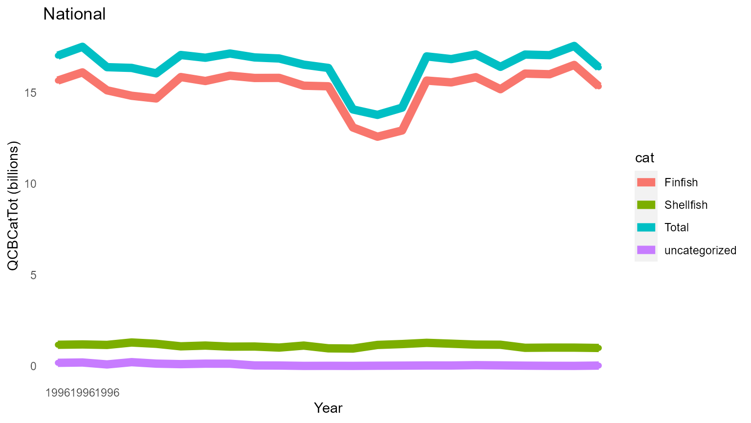
7. Figures

Here are a few figures that come out of this analysis!

Some come already in convient grids…

gridfigures_list$`000_All_byr2015_categoryPI_Total`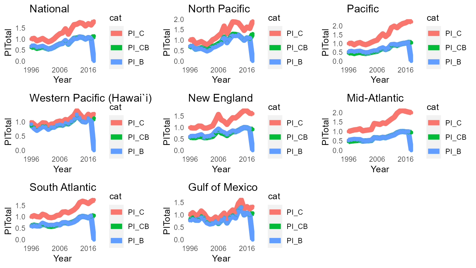

gridfigures_list$`000_All_byr2015_categoryQ_CB_Q`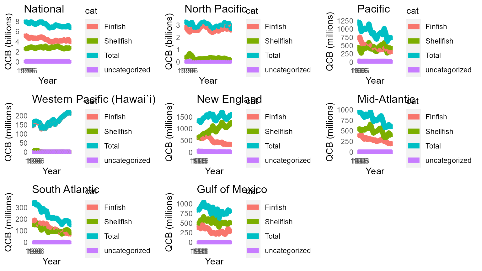

And in single plots!

figures_list$National__PI_Finfish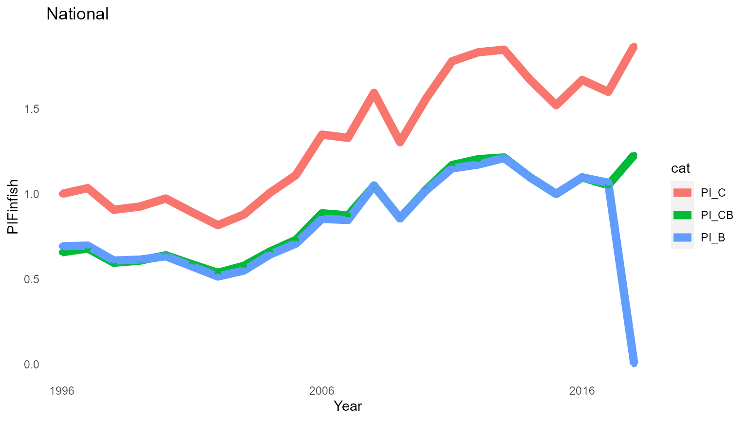

figures_list$National__Q_CB_CatTot_QCatTot